Objectives:
The purpose of this lab is to gain experience in working with vector quantities. The lab involves the demonstration of the process of the addition of several vectors to form a resultant vector. Graphical solutions for the addition of vectors will be carried out.
Equipment:
Force table with pulleys, ring and string.
Metric ruler, protractor, graph paper
Background:
If several forces with different magnitudes and directions act at a point its net effect can be represented by a single resultant force. This resultant force can be found using a special addition process known as vector addition.
Figure 1
First, let’s consider the process of vector addition by graphical techniques. Figure 1 shows the case of two vectors A and B, which are assumed to represent two forces. Using the “parallelogram method”, we draw a line from the tip of vector A parallel to B and equal in length to B. Let’s denote this line as vector B||. The resultant R of the vector addition of A and B is found by constructing the straight line from the point at the tail of vector A to the tip of the newly constructed vector B||.
In the process of vector addition, each vector to be added is first resolved into components as shown in Figure 1. The components along each axis are then added algebraically to produce the net components of the resultant vector along each axis. This leads to the following:
Rx = Ax + Bx = Acosq1 + Bcosq2
Ry = Ay + By = Acosq1 + Bcosq2 (1)
R = sqrt{[R(x)]^2 + [R(y)]}
Furthermore, the angle q that the resultant R makes with the X axis is given by the following:
theta = arctan[ R(y) / R(x)] (2)
The nonzero resultant force accelerates the system; hence, another force must be applied to to produce an equilibrium. If FA and FB are two known forces (represented by vectors A and B) applied to an object, they will have an resultant force (represented by the vector R). A force equal in magnitude and opposite in direction to R must be applied to keep the object in equilibrium. The force applied in order to produce the equilibrium is called the “equlibrant force. ”
Experimental Procedure:
We will use an instrument called the Force Table. A ring is placed around a pin in the center of the force table. Strings attached to the ring pull it in different directions. The magnitude (strength) of each pull and its direction can be varied. The magnitude of the string tension (force) is determined by the amount of mass that is hung from the other end of the string. The value of the pull (force) is mg, where g = 9. 81 m/s2 (recall Fw = mg). The force table allows you to demonstrate when the sum of forces acting on the ring equals zero. Under this equilibrium condition, the ring, when released, will remain on the spot.
Mount the Force Table in parallel to the working desk (horizontal position). Be sure that it is level.
Appendix
Experimental (trial and error) Method:
Add the required third force F3 calculated from the above methods to balance the other two forces. The ring should remain centered. If not, then change the direction and/or amount of the third force until it does. This balancing force is called the equilibrium force and it is equal in magnitude and opposite in direction to the resultant force of F1 and F2. Note the difference between the values and directions of F3 that you obtained experimentally and theoretically (using graphical and component methods).
Parallelogram Method:
Using a protractor and a ruler, draw arrows to represent the forces F1 and F2. Remember that you must choose a scale so that the length of each arrow is proportional to the magnitude of the force, and the direction of each arrow must be the same direction as the force it represents. Use either head-to-tail method or parallelogram method to draw an arrow that represents the resultant of the vectors. Measure the length of the arrow, determine the magnitude (size) of the resultant and its direction. To balance F1 and F2, you will need to apply a force F3 whose magnitude is equal to this resultant force, but opposite in direction.
Component Method:
With your calculator, determine the x and y components of F1 and F2. Remember that Fx = Fcos q and Fy = F sin q. Find the x and y components of the resultant from the sum of x and y components. Draw a right triangle with x and y components as sides, and the hypotenuse representing the resultant. Calculate the magnitude of the resultant from the square root of (Rx2 + Ry2). Calculate the direction of the resultant by using q R = tan-1 (Ry/Rx). Does this result agree with the graphical method?
Experiment with two forces:
- Place a pulley at the 30o mark on the Force Table and place a total of 0. 35 kg (which includes 0. 05 kg of the mass holder) on the end of the string. Place a second pulley at 130o mark and place a total of 0. 25 kg (including 0. 05 kg of the mass holder). Calculate the magnitude of the forces produced by these masses and record them in Table 1.
- From the value of the equlibrant force, determine the magnitude and direction of the resultant force and record them in Table 1.
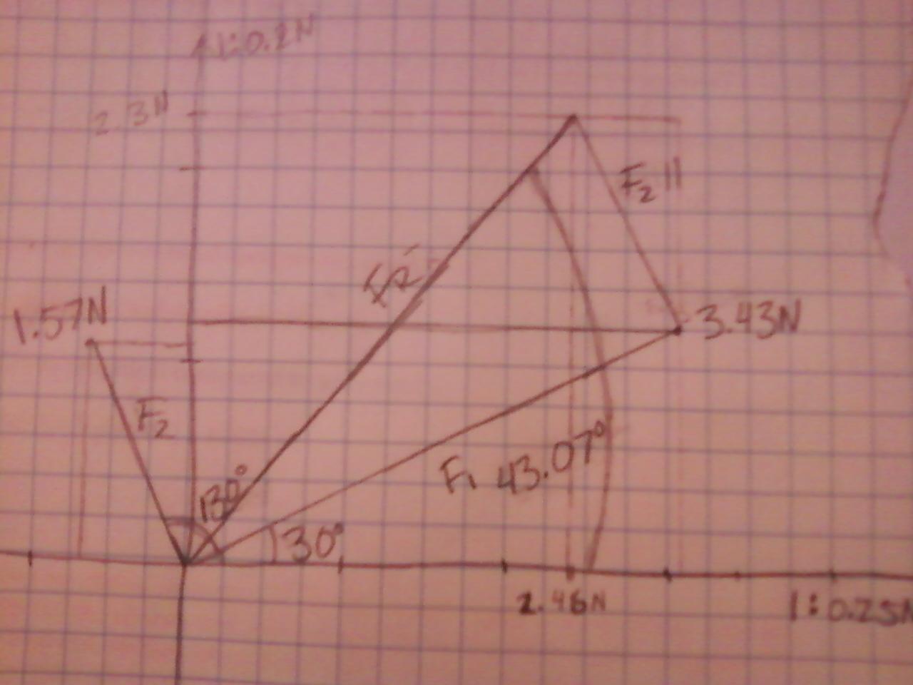
Calculations: - Find the resultant of these two applied forces by scaled graphical construction using the parallelogram method (See Appendix). Using a ruler and a protractor, construct vectors whose scaled length and direction representF1 and F2. A convenient scale might be 1 graphical division = 0. 1 N. Read the magnitude and direction of the resultant from your graphical solution and record them in Table 2.
- Using equation 1, calculate the components of F1 and F2 and record them into the analytical solution portion of Table 3. Add the components algebraically and determine the magnitude of the resultant by the Pythagorean Theorem. Determine the angle of the resultant. (See Appendix)
TABLE 1
Force
F1
F2
Equilibrant F
Resultant F
F1
F2
Equilibrant F
Resultant F
Mass (kg)
0.25
.035
0.358
0.358
0.25
.035
0.358
0.358
Force (N)
3.43
x = 2.97
y = 1.715
1.57
x = -1.01
y = 1.2
3.51
x = -1.96
y = -2.915
3.51
x = 1.96
y = 2.915
3.43
x = 2.97
y = 1.715
1.57
x = -1.01
y = 1.2
3.51
x = -1.96
y = -2.915
3.51
x = 1.96
y = 2.915
Direction
30 degrees
130 degrees
236.08 degrees
56.08 degrees
30 degrees
130 degrees
236.08 degrees
56.08 degrees
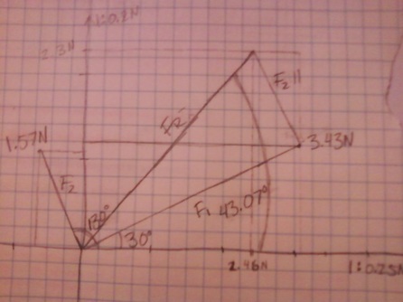
TABLE 2: Graphical Solution
Force
F1
F2
Resultant F
F1
F2
Resultant F
Mass (kg)
0.25
0.35
0.344
0.25
0.35
0.344
Force (N)
3.43
1.57
3.37
3.43
1.57
3.37
Direction
30 degrees
130 degrees
43.07 degrees
30 degrees
130 degrees
43.07 degrees
Table 3: Analytical Solution
Force
F1
F2
Resultant F
F1
F2
Resultant F
Mass (kg)
0.25
0.35
0.358
0.25
0.35
0.358
Force (N)
3.43
1.57
3.51
3.43
1.57
3.51
Direction
30 degrees
130 degrees
56.08 degrees
30 degrees
130 degrees
56.08 degrees
X component (N)
2.97
-1.01
1.96
2.97
-1.01
1.96
Y component (N)
1.715
1.2
2.915
1.715
1.2
2.915
Error Calculation:
Percent error magnitude graphical compared to analytical =
[(Graphical – Analytical)/Analytical] x 100% =
F1 : [(3.43 – 3.43)/3.43] x 100% = 0%
F2: [(1.57 – 1.57)/1.57] x 100% = 0%
FR : [(3.37 – 3.51)/3.51] x 100% = 3.99%
Discussion:
Percent error magnitude graphical compared to analytical =
[(Graphical – Analytical)/Analytical] x 100% =
F1 : [(3.43 – 3.43)/3.43] x 100% = 0%
F2: [(1.57 – 1.57)/1.57] x 100% = 0%
FR : [(3.37 – 3.51)/3.51] x 100% = 3.99%
Discussion:
- What sources of error could exist to account for differences between calculated and graphical analysis results?
| force_table_lab_revised1.doc |
| force_graph.jpg |
