Objectives:
1.Create a Displacement vs. Time graph and match your graph with actual motion.
2.Gain competence in the use of motion detector and related equipment.
3.Understand the relationship between position vs. time, velocity and acceleration.
Materials:
TI-84 Calculator-Based Lab Unit (CBL-II)
Motion detector
Meter stick
Computer with LoggerPro software
Procedure:
Part I –
1.Develop a position vs. time story that describes a body in motion incorporating at least the following four types of motion.
i.standing still
ii.moving with constant velocity
iii.moving with variable negative velocity
iv.moving with variable positive velocity
2.Illustrate the story on a position vs. time graph. Use a legend to cross reference sections of the graph with the corresponding sections of the story.
3.Underneath the graph, write instructions for moving in front of the motion detector according to the graph you have drawn (see page 2 for example).
Part II – AT THE LAB STATION IN CLASS WITH A PARTNER
4. Measure out and mark meaningful locations on the floor and practice the motion needed to create the position vs. time graph.
5. Now it’s time for you to match your physical motion to your group’s descriptive motion graph. You have 3 attempts to match it as best you can. Save a copy best graph your motion creates and reproduce this graph using LoggerPro.
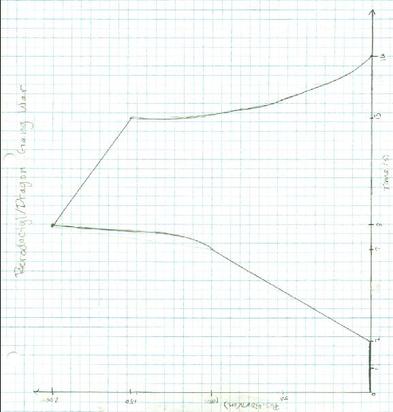
It was a sunny day in the land of Scisyhp, and the pterodactyl-samurai were being attacked by the dragon-wizards in an epic gang war. They were at opposite ends of the 200 meter marsh, glaring at each other for 2 seconds. Samurai flier BC signaled his pterodactyl—George—to fly directly at the lead wizard—Melvin—on his dragon—Billy Bob—at a light and steady pace of 20 meters per second for 5 seconds because the marsh was quite large and BC did not want his pterodactyl to tire. Halfway across the marsh, George began to increase his velocity at a constant 100 meters per second pace for one second in an attempt to hit Billy Bob with maximum momentum. He spun rapidly, achieving a constant velocity of 10 meters per second for 5 seconds and then increased his velocity 50 meters per second for 3 seconds as Billy bob spurted fire at him, in an effort to ensure self preservation. Sadly for the pterodactyls, it was all downhill from there. However, luckily for George and his Samurai, they returned to the pterodactyl base safely.
1 second = 2 seconds, 1 meter = 4 meters
1. With the book held in front of the motion detector, stand still for 1 second.
2. Gradually back up 1 meter at a constant velocity for 2.5 seconds.
3. Accelerate 1 meter for 2.5 seconds.
4. Immediately reverse direction and move back towards the motion detector for 0 .5 meters in 2.5 seconds.
5. Accelerate and cover 1.5 meters in 1.5 seconds to end at the initial position in front of the motion detector.
| motionlab.doc |

Time (Seconds)
0.5
1
1.5
2
2.5
3
3.5
4
4.5
5
5.5
6
6.5
7
7.5
8
0.5
1
1.5
2
2.5
3
3.5
4
4.5
5
5.5
6
6.5
7
7.5
8
Position
0.167428
0.182422
0.289598
0.550597
0.842971
1.13895
1.43577
1.93472
2.48282
2.59472
2.42729
1.76119
1.04733
0.395941
0.132721
0.133276
0.167428
0.182422
0.289598
0.550597
0.842971
1.13895
1.43577
1.93472
2.48282
2.59472
2.42729
1.76119
1.04733
0.395941
0.132721
0.133276
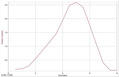
Data Analysis: Discuss differences between the descriptive graph and the graph generated by the motion detector. What are the reasons for the differences?
Many differences are apparent between the descriptive and generated graphs, but the noteworthy discrepancy between the two is affect of theoretical motion compared to applied motion. In the descriptive graph the motion is not sufficiently described because various actions—like the reversal of direction—are considered to take zero time to occur, where in the application of the motion, factors—such as the need for time to change direction—are accounted for. One of the discrepancies displayed between the two graphs is at the peak of the graphs; in the descriptive graph, theoretical time is taken into account and a sharp angle displays an instantaneous reversal of direction at 7 seconds. In the generated graph, a more realistic explanation of the motion is portrayed in the smooth curve at the peak; the generated graph demonstrates the necessary time needed to stop and reverse direction that the descriptive graph lacks.
Another difference exists in the initial movement between the two graphs. In the descriptive graph the person moving remains stationary and, from this stationary position, immediately enters into the constant velocity needed in the given scenario. However, the generated graph accounts for the initial build to the needed velocity that the descriptive graph does not take into account. Overall, the generated motion graph is more accurate in its description of the motion portrayed in the “Scisyhp” than the descriptive graph. It recorded smoother movement transitions that the descriptive graph simply did not take into account. The generated graph displayed the more applicable graph compared to the theoretical, descriptive graph.
Conclusion: Develop a conclusion that addresses the objectives of the lab.
Through graphical representations of the character in our story, this lab allowed us to familiarize ourselves with representations and analysis of motion. It enabled us to examine the difference between theoretical and applied motion and create a position versus time graph exemplifying the various position functions. We learned the variations on position versus time graphs and the different patterns the function curve aligns itself to with respect to velocity and acceleration. The motion detector illustrated how sharp angles in motion graphs are strictly theoretical and are translated into curves when carried out physically. This lab made the position versus time graphs more applicable because it enabled us to create motion off of which to base our graphs.
